Data Attribution for Diffusion Models

Written by Alex Cohen and Logan Engstrom.

Introduction

A fundamental problem we face when building machine learning systems is that of predicting counterfactuals about model behavior. For example, we may want to answer questions like: “What training data caused my model to fail?” or “What training data should I add to improve my model?” To solve these kinds of questions we turn to predictive data attribution, in which the goal is to predict how the output of a model will change if it is trained on a different training dataset. In this work, we aim to apply recent advances in data attribution (which can nearly perfectly calculate how models will change if given samples are dropped) to understand how training images contribute to generate new samples in diffusion models. Diffusion models are a particularly important (and newly popular) class of machine learning methods in which we want to understand the impact of training data.

Data attribution—which has been studied in various forms across domains from statistics to computer science since the 1960s [3, 4] —concerns the problem of understanding how the choice of training data changes model behavior. This primitive is widely applicable; for example, it is an important building block in downstream applications like model debugging/data selection (e.g., “how would the model output change if we did not train on this data?”) and data valuation (e.g., “how important was this training data for forming this model output?”). This field is particularly important in the context of image generation models for both legal and economic reasons. After all, diffusion models train on data generated by existing market players (e.g., artists) to produce outputs (e.g., new art) used in commercial contexts [13]. Data attribution for image generation in diffusion models has been a focus of recent work [5, 6]. In this problem, the goal is to, given a specified set of samples to drop, understand how the likelihood of a given sample being generated changes after dropping that set of samples. People have also used likelihoods to study membership inference in diffusion models [2], or answering the question of if a given sample was included in the training set. However, these works have two main limitations. First, they evaluate approximate empirical likelihoods of the diffusion model, rather than true likelihoods. Second, they have much room for improvement in accuracy: their estimates of how models will behave after dropping certain training data only weakly correlate with how models actually behave after dropping such data. We address both of these limitations; our contributions are as follows:

Using a differentiable likelihood function for data attribution: While diffusion model likelihoods have been used in the past in various contexts [2, 7, 9], we are the first to use a differentiable likelihood function for data attribution in diffusion models. Since computing this likelihood involves solving another differential equation, we can calculate the gradient of this likelihood by either solving the continuous adjoint equations or backpropagating through the solver, giving us an exact and efficient method [8, 9]. We backpropagate through the solver and use recursive/binomial checkpointing to avoid memory issues [14].
Near-optimal data attribution with the influence function: We apply metagradients [11] to calculate near-optimal data attributions for diffusion modeling via the influence function [10]. In contrast, we find that existing baselines often cannot predict likelihoods better than random. This method uses gradients of the training routine to calculate the exact influence function estimate of how dropping data would change model outputs. By combining gradients through training with gradients of the likelihood of sampling a given image we near perfectly compute how the likelihood of a given sample changes when we drop certain training data.

Methods

In what follows, we detail the goal, then the methods and experiments we use to achieve the goal.

Weighted Data Attribution

We first define the goal. As setup, suppose that we have a pool of $n$ training data samples $\{z_i\}_{i=1}^n$, each of which has a weight $w_i$ multiplying its loss during training. Furthermore, suppose our learning algorithm $A$ maps data weights $w$ to the downstream parameters. Let $\phi_x$ map parameters to the likelihood of a given generation $x$ (fixed), and finally let $f = \phi_x \circ \mathcal{A}$.

In this setup, setting a weight $w_i = 0$ removes the data from training, and $w_i = 1$ keeps the data during training. Our goal is to predict how removing a given training point $z_i$ changes the likelihood of generating a given sample. To formalize this notion, let $w^{-i}$ be the weight vector for which the $i$th slot is $0$ and all the remaining slots are $1$. Then our goal is to, for any training sample $i$, estimate $f(w^{-i})$.

To give an instructive example of this setup, we detail the diffusion learning setting we study in this work. Here, the training pool is $n$ inputs from the distribution of interest $z_i = \mathbf{x}_i \in \mathbb{R}^d$; the learning algorithm $\mathcal{A}$ fits a diffusion model in an iterative fashion, i.e., it takes the form

\[\mathcal{A}(w) := s_T \quad \text{for} \quad s_{t+1} := h_t(s_t, \mathbf{g}_t(s_t, w)) \quad \text{ and } \quad \mathbf{g}_t(s_t, w) := \sum_{i\in B_t} w_i \cdot \nabla_{s_t} \ell(z_i; s_t).\]

Above, $s_t$ is the optimizer state (including model parameters), which is iteratively updated by a step function $h_t$ starting from a fixed initial state $s_0$ (in our diffusion modelling setting these quantities represent the ADAM optimizer steps and state). We denote the number of training steps by $T$; $B_t \subset [N]$ is a minibatch sampled at step $t$; and $\ell(z_i; s_t)$ represents the loss on sample $z_i$ given optimizer state $s_t$ (where our loss is the standard denoising loss). Then, the goal is to predict a model’s likelihood on a specific point $x$ via the likelihood function $\phi_x$. Then, $f(w) := \phi_{x} \circ \mathcal{A}$ maps a data weighting $w$ to the resulting model’s likelihood on a generation $x$. The vast majority of large-scale ML algorithms are iterative in this sense, and diffusion models are no exception.

Broad Strategy: The Influence Function

We will estimate the output of the model via the influence function calculated via metagradients [4, 3, 11]. This is exactly the Taylor expansion of $f$ starting at the all ones data weight:

\[f(w^{-i}) \approx f(1_n) + \frac{\partial f({w})}{\partial{w}}\bigg|_{w=1_n}^\top \left(w^{-i} - 1_n\right).\]

Previous work used this approximation to obtain near-optimal estimates of image classification model outputs [10]; in this work we aim to replicate this success for the likelihood of diffusion models generating a given sample. To do so, we need to be able to calculate the gradient above, which requires (via the chain rule since $f$ is a composition of both the likelihood of generating $x$ $\phi_x$ and the learning algorithm $\mathcal{A}$) both (a) a differentiable likelihood function $\phi_x$ (described above) and (b) a differentiable training method $\mathcal{A}$. The core of our work will be implementing both of these two building blocks in the context of score-based diffusion models.

Ingredient 1: A differentiable likelihood function $\phi_x$

In score-based diffusion models, the forward process is defined by an SDE that adds noise to smooth the data distribution, $p_{\text{data}}(x)$. The SDE is in the form:

\[d\mathbf{x} = \mathbf{f}(\mathbf{x},t)dt + g(t)d\mathbf{w}\]

At $t=0$, we have $p_0(x) = p_{\text{data}}(x)$, while at time $t=1$, we have $p_T(x) = \pi(x)$, a noise distribution, which depends on $f(x,t)$ and $g(t)$. There are many possible choices for $f(x,t)$ and $g(t)$, but usually they are chosen so $\pi(x)$ is analytically tractable. In this work, we use the variance exploding SDE, which has the form

\[d\mathbf{x} = \sigma(t)d\mathbf{w}\]

and we specifically use

\[d\mathbf{x} = 25^td\mathbf{w}.\]

To generate samples, we need to solve the reverse-time diffusion process from $t=1$ to $t=0$. This equation is given by:

\[d\mathbf{x} =[\mathbf{f}(\mathbf{x}, t) + g(t)^2\nabla_\mathbf{x}\log p_t(\mathbf{x})]dt + g(t)d\mathbf{w}.\]

In order to solve this equation, we just need the time-dependent score function $\nabla_\mathbf{x}\log p_t(\mathbf{x})$. We can estimate this with a score-based neural network model, $\mathbf{s}_\theta(\mathbf{x}, t)$, which in practice we accomplish with denoising score matching objective [12]:

\[\min_\theta \mathbb{E}_{t\sim \mathcal{U}(0, T)} [\lambda(t) \mathbb{E}_{\mathbf{x}(0) \sim p_0(\mathbf{x})}\mathbb{E}_{\mathbf{x}(t) \sim p_{0t}(\mathbf{x}(t) \mid \mathbf{x}(0))}[ |s_\theta(\mathbf{x}(t), t) - \nabla_{\mathbf{x}(t)}\log p_{0t}(\mathbf{x}(t) \mid \mathbf{x}(0))|_2^2]].\]

The differentiable likelihood function: While this SDE formulation does not directly enable exact likelihood calculation, continuous normalizing flows models, which are based on ODEs, do enable exact likelihood calculation. (Note: popular diffusion moodel variants such as denoising diffusion probabilistic models (DDPMs) can be expressed in the same SDE framework as score-based diffusion models to enable exact likelihood calculation [12]. Furthermore, we can convert the SDE into an ODE by using the associated probability flow ODE, which shares the same marginal distribution at each time step as the SDE [7].

Now, to get the change in log probability of $\mathbf{x}$ undergoing the transformation given by the probability flow ODE, we can leverage the instantaneous change of variables formula, which gives another equation describing the change in log probability of $\mathbf{x}$:

\[\ln p_0(\mathbf{x}(0)) = \ln p_1(\mathbf{x}(1)) + \int_0^T \nabla \cdot \bigg(-\frac{1}{2}g(t)^2\mathbf{s}_{\boldsymbol{\theta}}(\mathbf{x},t)\bigg)dt.\]

Since the divergence term in the above equation is expensive to compute, most people use the Skilling-Hutchinson’s trace estimator to approximate it [12]. However, we use the exact divergence in this work with and solve the equation with recursive checkpointing to avoid memory issues [14]. The last step is to convert the log likelihood to bits/dimension (BPD), a commonly used unit for evaluating diffusion models. BPD for generative models essentially measures the average number of bits the model needs per pixel to represent the image. This quantity is more useful than the log likelihood, as it is normalized by the dimensions of the data, which allows for comparison between different models and datasets. In addition, BPD is a more interpretable unit for the likelihood of a sample, as it represents the amount of information compression the model achieves. A normal 8 bit grayscale image requires 8 bits/pixel, so a lower BPD, say of 2, indicates that the model has achieved a compression of 4x. Thus, a lower BPD corresponds to a higher likelihood of the sample, which can be seen in the conversion below.

\[\text{bits/dim} = -\frac{\ln p_{\boldsymbol{\theta}}(\mathbf{x})}{D \ln 2},\]

where $D$ is the dimension of the data (number of pixels times number of channels).

Ingredient 2: Metagradients

The second ingredient we need is a way of calculating the influence—i.e., the gradient of the likelihood function with respect to the data weights (as described in the first part of this section). To do so, we use MAGIC [10], a recently developed method for data attribution that calculates closed-form influence function with the metagradient [11] to calculate the gradient of the likelihood function with respect to the data weights. The metagradient is the gradient over model training, i.e., the gradient of a function of model training with respect to a setup quantity in model training (like data weights). In particular, the method of [11] operates by computing the gradient using large-scale autodifferentiation through the entire training process. Naively this approach is infeasible, as it requires storing much of the training process in memory, which is not possible for large-scale model training; the method uses an elaborate recursive checkpointing scheme to avoid this issue. Naively, the metagradients obtained with this method is too unstable to be useful; however, the authors of [11] show that by carefully modifying the training process, we can obtain a stable metagradient that is useful for data attribution. In this work, we simply grid over the learning rate schedule, batch size, and ADAM hyperparameters to find a set of hyperparameters that yield a stable metagradient (as described in [11]).

Putting it all together

To summarize, we calculate the influence function of the likelihood of a score-based diffusion model generation via the following steps (Figure 1):

Assign one weight $w_i$ to each MNIST training sample.
Train a score-based diffusion model based on the variance exploding SDE and the denoising score matching objective on the MNIST training set.
Compute the log likelihood of a query image in BPD.
Use metagradients to calculate the influence of each training sample on the likelihood of the query image.

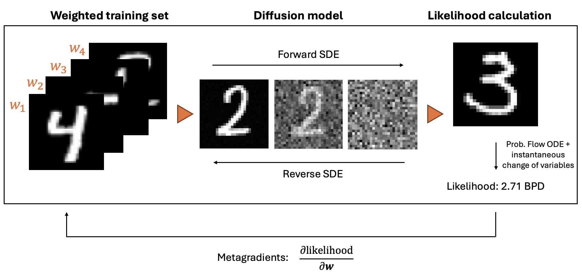
Figure 1: Overview of our method. We train a score-based diffusion model on a training set of images, then use metagradients to calculate the influence of each training sample on the likelihood of a query image.

Experiments

We perform our experiments on MNIST as we have few GPU resources available for this project. We hope that our results will reflect how our method will perform if scaled to larger settings.

The first experiment that we conducted was to verify that the likelihood of generating images, as measured in BPD, is a useful quantity to use for predictive data attribution in diffusion models. This is not obvious because the characteristics that are captured through the likelihood are unknown [1]. In particular, while some previous work has used unconditional diffusion model likelihoods for certain tasks [2], other work has shown that conditional diffusion model likelihoods are not useful [1]. To test whether the likelihood of generated images is a useful quantity for predictive data attribution, we trained an unconditional diffusion model on MNIST then calculated the likelihood of generating MNIST training images, rotated training images, the average of multiple training images, and images generated from random noise.

After verifying that the likelihood of generating images is a useful quantity for predictive data attribution, we train a diffusion model on the entirety of MNIST, generate a sample, then train a new diffusion model on the entirety of MNIST minus a single training datapoint $i$, measure the likelihood of sampling the previously sampled image, then compare how this quantity compares with our influence function approximation. We repeat this experiment many times to ensure soundness and robustness across randomness, and compare with existing baselines [5, 15].

Results

Verifying Utility of Diffusion Likelihoods

Overview
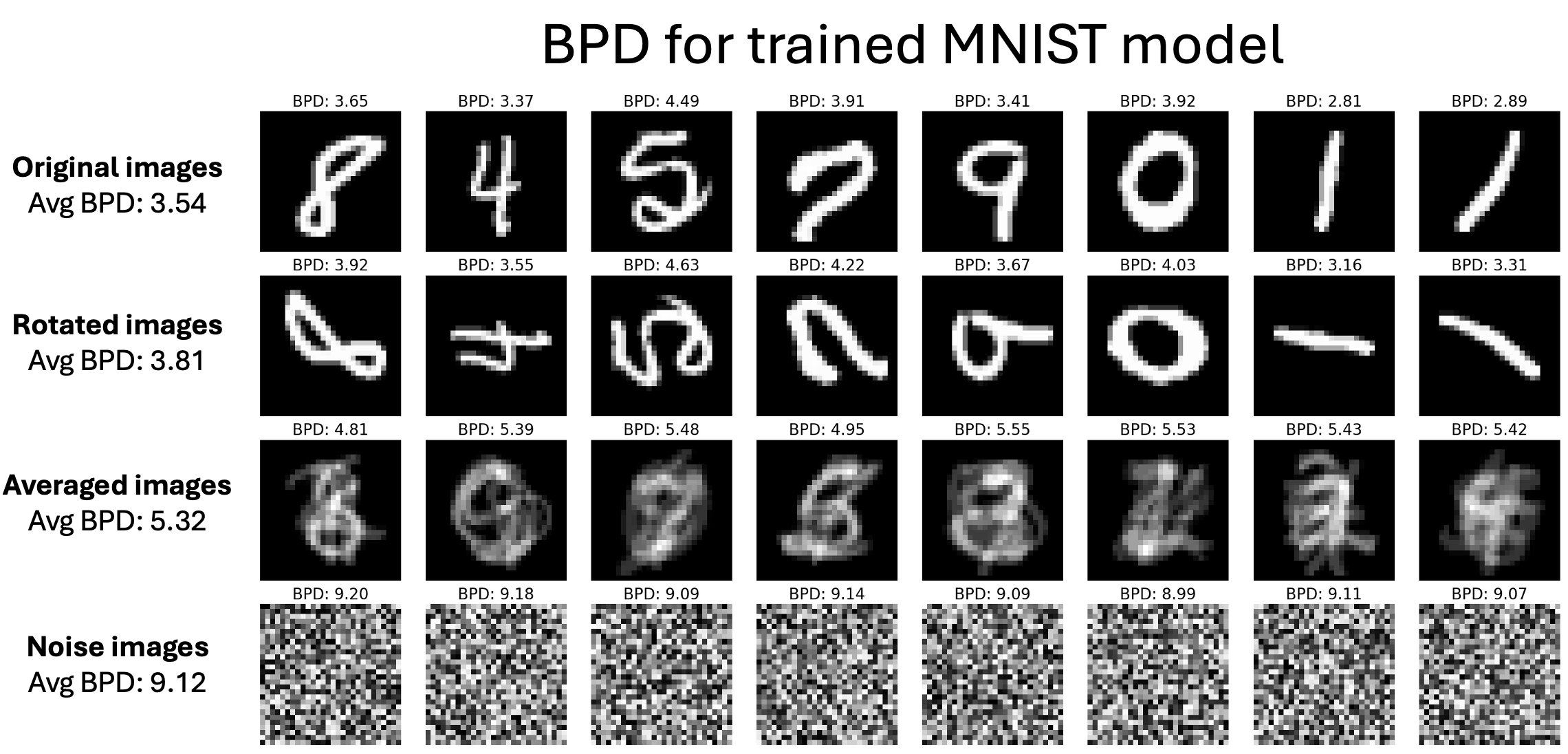
Figure 2: Comparison of bits per dimension (BPD) for different types of images. Lower BPD indicates higher likelihood of the model generating that image. Original MNIST images have lower BPD than rotated or averaged images, while random noise has the highest BPD.

In order to verify that the likelihood of generating images is a useful quantity for predictive data attribution, we trained an unconditional diffusion model on MNIST then calculated the likelihood of generating MNIST training images, rotated training images, the average of multiple training images, and images generated from random noise (Figure 2). For all examples, the original MNIST images have a lower BPD, or higher likelihood, than the rotated images, as expected. In addition, one of the examples includes a weird looking 5, which has the highest BPD, or lowest likelihood, of all the examples. On average, the original MNIST images have a BPD of $\approx 3.5$, while rotated images have a BPD of $\approx 3.8$. While this difference may not seem very large, given the fact that the MNIST images are 28x28 grayscale images, this corresponds to a dimension of 784, and thus a relative likelihood difference of $2^{(3.5-3.8)*784}$, which is $\approx 10^7$. Thus, the model is $\approx 10^7$ times more likely to generate a non-rotated image than a rotated image. The averaged images show an even more drastic difference, with an average BPD of $\approx 5.32$. However, the rotated and averaged BPD values are still much lower than the standard 8 bit grayscale images, indicating that the model can still identify features of these images that are similar to the digits in the MNIST training set. Finally, the random noise images have an average BPD of $\approx 9.12$, which is even larger than standard 8 bit grayscale images, indicating that the random images are less likely according to the model than the baseline of when all possible images are equally likely. We can also interpret these values as a measure of how “in-distribution” images are. Thus, these results seem to indicate that the BPD values are meaningful and we can use this quantity to measure the influence of a sample on the model.

MAGIC Nearly Perfectly Predicts Model Behavior

Overview
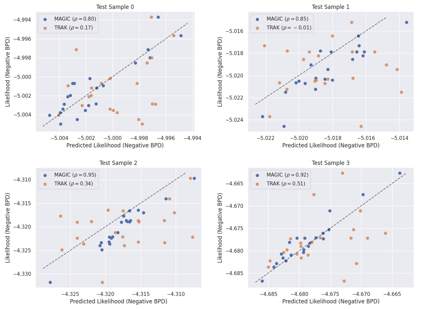
Figure 3: Comparison of MAGIC predictions of the likelihood for 4 test images after removing 1% of the training set. We label the plots with $$\rho$$, or the Spearman rank-correlation between the observed and predicted quantities. MAGIC predictions are strongly correlated with the true likelihoods, while the baseline TRAK predictions are only weakly correlated at best.

In this section we verify that our method MAGIC can accurately predict the likelihood of a generated image when a training sample is removed. In particular, we choose 4 different random test images, then repeatedly retrain models with $1%$ of the training set removed. For each of these retrained models, we calculate the likelihood of the test images, then compare this likelihood with the predicted likelihood from MAGIC (and TRAK, the best existing baseline). We find that while MAGIC predictions are strongly correlated with the true likelihoods (reaching typically in the sampled images a Spearman rank-correlation of $\rho \approx 0.9$), the TRAK predictions are only weakly correlated at best (reaching typically $\rho \leq 0.3$).

Visualizing Most Influential Training Samples

Overview
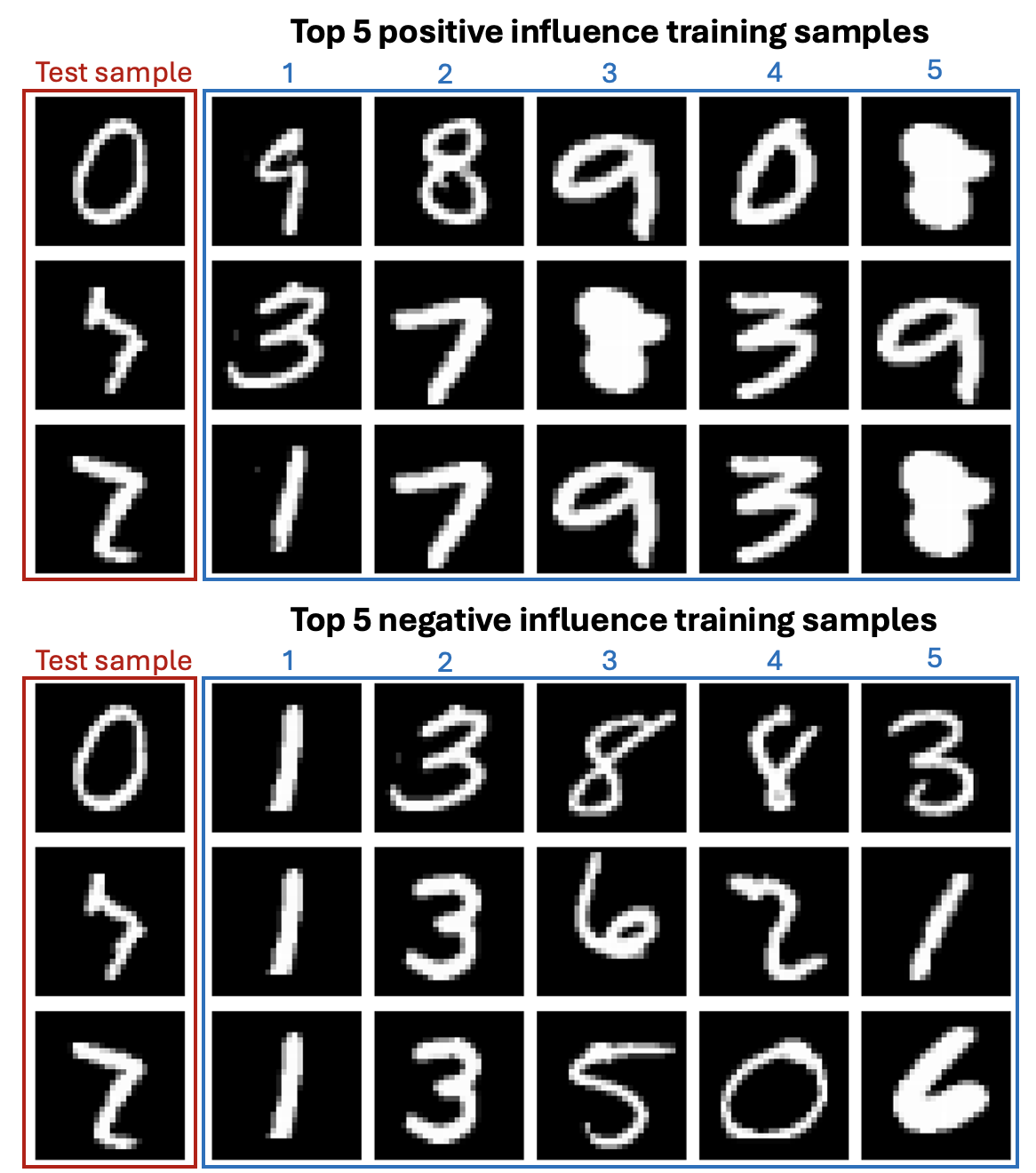
Figure 4: Visualization of the most positive and negative influential training samples for a test image.

We can also use the metagradients to visualize the most influential training samples for a given test image (Figure 4). The most positive influential samples are samples that are predicted to increase the likelihood of the test image, while the most negative influential samples are samples that are predicted to decrease the likelihood of the test image. Unexpectedly, we find that the most influential training samples generally do not look similar to the test image. In addition, the top influential samples are shared across different test images. We also notice that the “1” digit is the most negative influential digit for all test images, which is interesting because we also find it to be the digit that has the highest likelihood of being generated by the model (Figure 2). These results raise import questions for future work, including (i) Why are do certain training samples have a high influence on very different test samples; (ii) What features of the images have a strong influence on their likelihoods; and (iii) Does this same behavior also occur in conditional diffusion models or diffusion models on more complex datasets?

Discussion

Overall, we have successfully demonstrated our novel insight that the likelihood of a generated image is a useful quantity for predictive data attribution in diffusion models. Furthermore, we have shown that the metagradients of the influence function can near perfectly predict the change in likelihood of a generated image when a training sample is removed. We have also shown that the specific training images that have the most influence on a given test image are shared across different test images, and are not necessarily similar to the test image.

However, we would like to stress that this work is not without its limitations. First, we only tested our method on MNIST, a very simple dataset, and we do not yet know how well our method will perform on more complex datasets. Second, we only tested our method on unconditional diffusion models, but most real-world diffusion models are conditional, like text-to-image models. Third, our method is very expensive; it costs approximately 4x the training time of a standard diffusion model to calculate the influence function. However, with more GPU resources and more time, we are confident that we can extend our method to more complex datasets and conditional diffusion models.